 If you haven’t noticed by now, two of my big passions are spatial data wrangling and football (soccer). I’m quite surprised that it’s been three years (2015) since I delved into this subject, so here’s an update for 2018.
I haven’t (yet) managed to get hold of any player tracking data, but I do have the location of stadiums and you can generate a surprising amount of interesting facts and trivia with just that. So this article explores data integration through the geography of football stadiums in England and Wales.
I’ll start out with the statistics, and then mention the methodology below that. But if you were drawn here by the football rather than as a regular reader, then you should know I’m using a product called FME. FME is a Data Integration platform, with the capability to read and process data in multiple formats and types. It’s especially efficient on spatial datasets, such as used in GIS and CAD systems. So if you too wrestle with data on a regular basis, please do check it out.
And now on to the football…
![]()
Source Data
So the source data I used for this is very simple. It’s just a list of English football teams and their home grounds stored in a comma-separated text file:
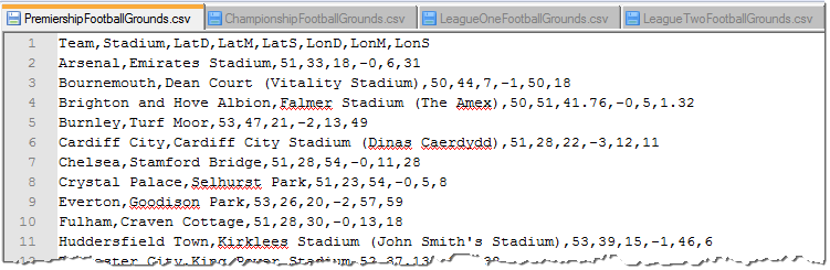
Notice that I have the latitude and longitude (as degrees, minutes, seconds) for each ground. I also have a dataset of Ordnance Survey open data from which I extracted roads (specifically A Roads, B Roads, and motorways).
Here are links to use if you want to download the data for yourself:
- Source List of Stadiums (CSV Format)
- Ordnance Survey Open Data (Link to OS website. Shapefile and GML formats available)
I used FME to turn the CSV into a true spatial dataset and incorporated it with the OS data to generate as many statistics as I could think of, as you can see below…
![]()
Away Game Journeys (Individual)
If I know where stadiums are, and I have a road network – plus I know which team is in which league – I can very easily use FME to calculate the longest and shortest individual journey during the season. Here’s a table of the results:
| League | Shortest Journey | Longest Journey |
|---|---|---|
| Premier | Liverpool vs Everton (3 km) | Bournemouth vs Newcastle (1,052 km) |
| Championship | Sheffield United vs Sheffield Wednesday Aston Villa vs Birmingham (both 11 km) |
Swansea vs Middlesborough (887 km) |
| League One | Blackpool vs Fleetwood Town (28 km) | Plymouth vs Sunderland (1,246 km) |
| League Two | Oldham Athletic vs Bury (33 km) | Exeter vs Carlisle (1,081 km) |
Incidentally, all numbers are in kilometres, and include a journey by road from the home ground to each away ground, and back again.
Obviously, the reverse fixtures (e.g. Everton vs Liverpool) are the same distance, meaning that the two sides closest geographically have the same shortest journey. The two teams geographically most distant also have the same longest journey. But that doesn’t work for all other teams though; just because Southend’s shortest trip is Charlton, it doesn’t mean that Charlton’s shortest trip is Southend.
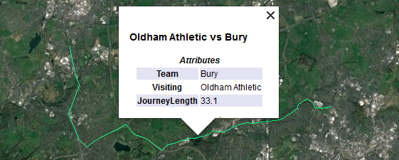
Anyway, here’s League Two’s shortest trip, between Oldham and Bury (and vice versa) as viewed in Google Earth:
I didn’t check, but I figure the longest possible fixture would be Plymouth vs Newcastle, at over 1,300km round trip. They aren’t in the same league, but if they draw each other in the cup, that’s the journey they face! To give some perspective to North Americans, Chicago is approximately 1,300km away from New York. For Australians, Sydney and Adelaide are pretty much 1,300km apart.
![]()
Away Game Journeys (Cumulative)
After calculating match distances all I need to do is add them together to get a cumulative amount of travel for the season. I think this is my favourite statistic. It shows how far each team travels to away matches, and how far a supporter who went to every away game would have to travel!
So I had FME calculate this for every team in all four of the English football leagues, for the 2018/19 season. From that I created a Google Earth KML dataset showing every single match, for each team in each league, and an Excel spreadsheet that summarizes the results. This is what the data for Charlton Athletic (for example) looks like in Google Earth (click to enlarge):
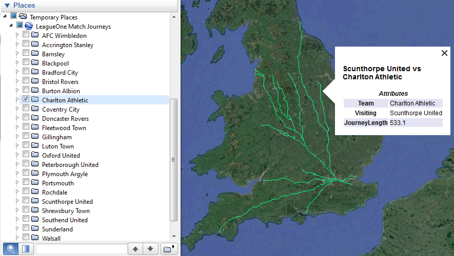
Each of the green lines is a separate away game, and they can be clicked on to see who the game is against and how long the return journey is. If you feel like it, please do download the file for your league and check out your team’s travels…
Downloads
Here are the links to use if you want to download the datasets for yourself:
- Premier League Match Journeys (Google KML)
- Championship Match Journeys (Google KML)
- League One Match Journeys (Google KML)
- League Two Match Journeys (Google KML)
- Match Journey Results Summary (Microsoft Excel)
Summary
Here’s a brief summary of the top/bottom three for each league, as recorded in the Excel dataset:
| Premier League | Longest | Premier League | Shortest | ||
|---|---|---|---|---|---|
| 1 | Newcastle United | 13,805 | Watford | 6,476 | |
| 2 | Cardiff City | 9,738 | Leicester City | 6,566 | |
| 3 | Bournemouth | 9,396 | Arsenal | 6,616 | |
| Championship | Longest | Championship | Shortest | ||
| 1 | Swansea City | 13,347 | Derby County | 6,281 | |
| 2 | Ipswich Town | 11,889 | Nottingham Forest | 6,443 | |
| 3 | Middlesborough | 11,876 | Sheffield United | 6,610 | |
| League One | Longest | League One | Shortest | ||
| 1 | Plymouth Argyle | 18,165 | Coventry City | 7,436 | |
| 2 | Sunderland | 15,021 | Burton Albion | 7,474 | |
| 3 | Portsmouth | 12,250 | Walsall | 7,639 | |
| League Two | Longest | League Two | Shortest | ||
| 1 | Carlisle United | 15,394 | Notts County | 7,252 | |
| 2 | Exeter City | 14,347 | Port Vale | 7,415 | |
| 3 | Yeovil Town | 12,016 | Northampton Town | 7,551 |
So, for example, Ipswich fans would need to travel 11,889 kilometres to watch every away game; Port Vale fans would need travel only 7,415.
As a single table, the top/bottom five are:
| Team | Longest | League | Team | Shortest | League | ||
|---|---|---|---|---|---|---|---|
| 1 | Plymouth Argyle | 18,165 | League One | Derby County | 6,281 | Championship | |
| 2 | Carlisle United | 15,394 | League Two | Nottingham Forest | 6,443 | Championship | |
| 3 | Sunderland | 15,021 | League One | Watford | 6,476 | Premier | |
| 4 | Exeter City | 14,347 | League Two | Leicester City | 6,566 | Premier | |
| 5 | Newcastle United | 13,805 | Premier | Sheffield United | 6,610 | Championship |
Some interesting facts:
- The team with the shortest overall journey is Derby Country, even though they play four more games than Premier League teams.
- Notts County (7,252 km) travel much further than Nottingham Forest (6,443) even though their grounds are almost adjacent.
- Barnsley and Swindon Town are the only two teams whose travel is identical to the nearest kilometre (8,726 km)
Straight Line Distances
Another interesting fact is that straight line distances do not give the same results. So I figured that if I calculated road distance as a percentage of straight line distance, I’d get a measure of how well the road network suits each team. i.e. If there was a road from your stadium directly to each other team, in a straight line, the percentage would be 100.
So the closer to 100 the better, and the winners of that contest are – perhaps not surprisingly – London clubs:
| Team | Ratio Straight:Road Distances | League | |
|---|---|---|---|
| 1 | Arsenal | 111.08 | Premier |
| 2 | Millwall | 111.18 | Championship |
| 3 | West Ham United | 111.28 | Premier |
So step forward Arsenal. Your fans are best served by the road network, and have the least excuse to charter a helicopter to travel to matches! But on the other hand…
| Team | Ratio Straight:Road Distances | League | |
|---|---|---|---|
| 1 | Cardiff City | 117.45 | Premier |
| 2 | Swansea City | 116.97 | Championship |
| 3 | Fleetwood Town | 116.73 | League One |
Poor Cardiff. Their fans have the second-longest set of journeys in the Premier League (29th longest overall), and the road network takes them further from a straight line trip than any other team!
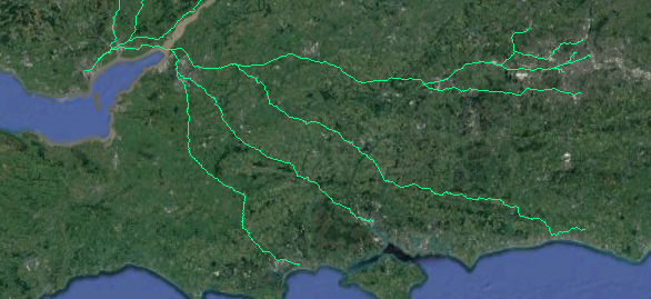
This screenshot of Google Earth shows how their journey to Bournemouth (for example) is far from a straight line trip.
This information is also in the Excel spreadsheet so you can check out your team of choice there. Newcastle United fans (for example) will find that although they come 88th out of 92 for shortest road distance, they are 20th as a percentage of straight line distance, meaning at least the road network is kind to them. Look at Northampton Town for an example of the opposite.
![]()
Visiting Every Ground
I know that some fans try to visit every ground in a single season. While I can’t figure out the best schedule to do that and watch a game at each ground (OK, I could, but I won’t) I can very easily use FME to tell you the shortest route to visit all of the grounds.
This is what is known as the Travelling Salesman Problem, and I’ve blogged about this before. Basically it’s a problem without a solution (unless you can prove NP=P or not). All you can do is iterate through the data again and again, looking for a shorter route.
I initially set FME to run through 100,000 iterations (100,000 different solutions). Then just to confirm the result I tried with 5 million iterations and then – because it was just running so fast – 100 million, and then one billion iterations. So take it from me, you’re unlikely to get a better result than this (click to enlarge):
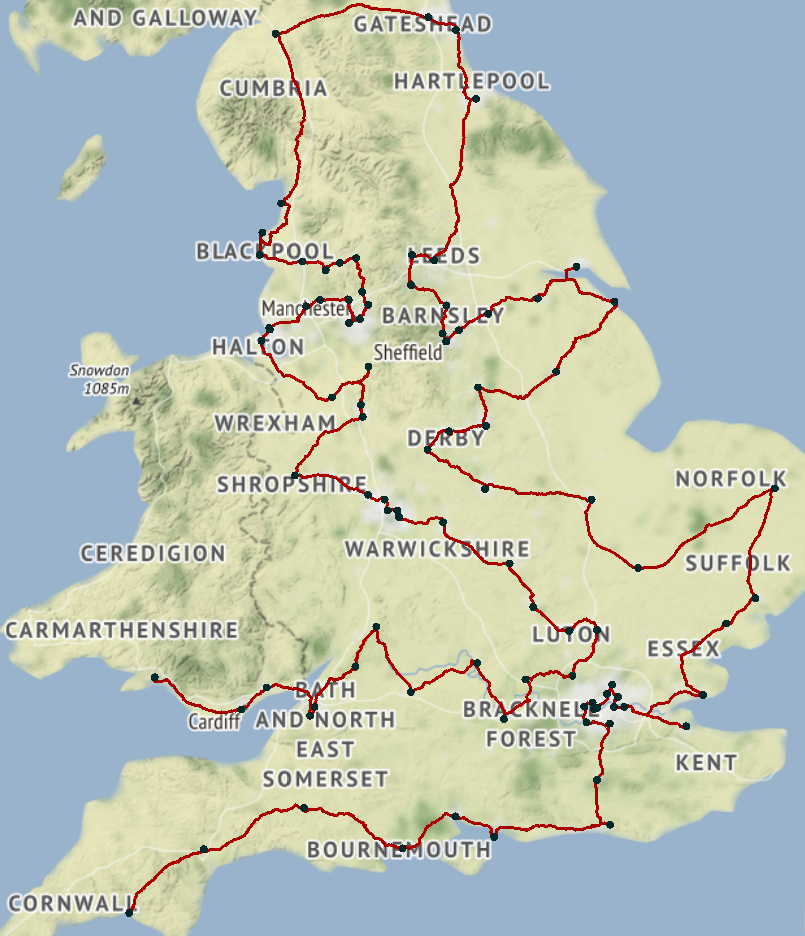
Map tiles by Stamen Design, under CC-BY-3.0. Data by OpenStreetMap, under CC-BY-SA
So your route starts at Plymouth, ends at Swansea – or vice versa – and covers 3,022.7 km of driving.
If you want to check it out, I’ve got the route available in KML, and through the magic of FME also in GPX, in case you feel like uploading it to a GPS device and travelling the route for yourself!
Downloads
- Shortest route to all grounds (Google KML)
- Shortest route to all grounds (GPX)
Know that I’m using A roads, B roads, and motorways only, to get as close to the stadium centre as possible. I allow a little leeway (up to 1.25km) because very few stadiums have a road run right to the ground, let alone through the centre circle!
![]()
Geographic Monuments
Firstly a quiz question for you. If you’re a geography geek, then you’ll know that the prime meridian – the line of zero longitude – passes through London at Greenwich, and divides the world into two hemispheres. So, here’s a good question for your next trivia quiz: how many English football grounds lie east of the prime meridian, and can you name them? The answer is further below.
In the meantime… around the world there are many monuments that denote the “most westerly” or “the centre of” or something similar. So, if English football were to create monuments, where would they be? That’s another fairly simple task with FME.
If we’re just looking at the top four professional leagues, then obviously geographic statistics change over time, because teams regularly get relegated out of, or promoted in to, the league system. Plus there are also teams regularly moving to a new stadium. So these figures are good for 2018 only, but the geographic extremes are fairly predictable and (I imagine) unlikely to change:
| Record | Team | League |
|---|---|---|
| Most Northerly | Newcastle United | Premier |
| Most Southerly | Plymouth Argyle | League One |
| Most Easterly | Norwich City | Championship |
| Most Westerly | Plymouth Argyle | League One |
Plymouth there, with the distinction of being the most southerly and most westerly club; no wonder they have the longest away journeys. As you would expect, these teams are mostly coastal, or close to the coast. Newcastle just scrapes past Sunderland and Carlisle for the most northerly.
Incidentally the reason I think these won’t change is that none of the above can be relegated from League Two, and no team in the National League Premier that could be promoted is more extreme. Dover and Gateshead come close, but can’t beat the most easterly and northerly respectively. So those numbers are safe at least until the 2020 season.
The geographic centres of football are just as easy to calculate (it’s just the average of all stadium latitude/longitude numbers) and unsurprisingly all fall in the Midlands. They don’t fall on one particular stadium though; for example, the geographic centre of football in England is (drumroll…)
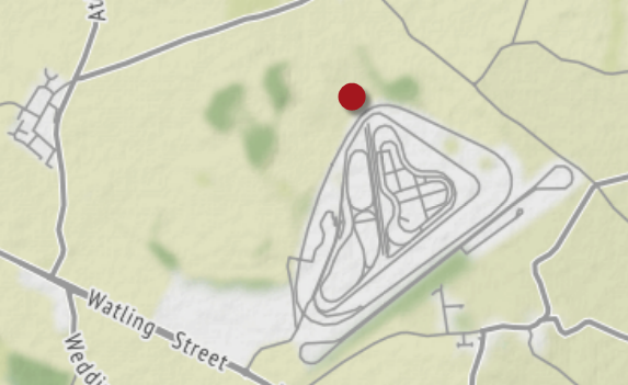
Map tiles by Stamen Design, under CC-BY-3.0. Data by OpenStreetMap, under CC-BY-SA
Well, it’s an obscure spot on the north border of the MIRA Technology Park, just off the A5, at Higham-on-the-Hill, near Nuneaton. So if you work in this park, you can say that you work at the geographic centre of English football! If we can’t get a monument there, we should at least have someone place a geocache.
Coincidentally, this is very close to a place called Lindley Hall Farm, suggested as the actual geographic centre of England; so the centre of English football is pretty much the centre of England itself. And it really is coincidental. Given the spread of teams the geographic centre was always going to be in the Midlands, but to be just 200 metres from the centre of England is a little surprising.
Incidentally, the closest team to this fabled spot: Coventry City. Coventry fans rejoice. Your stadium is literally the geographic centre of English football! In table form:
| Centre Of… | Nearest Town | Nearest Team |
|---|---|---|
| All Football | Higham-on-the-Hill (Leics) | Coventry City |
| Premier | Draycote (Warks) | Leicester City |
| Championship | Breedon-on-the-Hill (Leics) | Derby County |
| League One | Higham-on-the-Hill (Leics) | Coventry City |
| League Two | Hurley (Warks) | Notts County |
For the individual leagues, the nearest team is the nearest in that same league. It’s pure coincidence, but the geographic centre of all teams and the geographic centre of League One, is virtually identical, which is how Coventry get a double mention.
Finally for this section, the answer to the question above about the prime meridian. There are seven teams east of the prime meridian (so in the eastern hemisphere). They are Cambridge, Charlton, Colchester, Gillingham, Ipswich, Norwich, and Southend. Incidentally, West Ham also used to hold that unique distinction; but then they moved from Boleyn Park/Upton Road to the Olympic Stadium. Not a huge move in terms of distance, but in geographic terms it’s a completely different hemisphere!
Downloads
As with the other statistics, I have a dataset of information that you can download:
- Geographic Monuments to Football (Google KML)
![]()
Who Should You Support?
Football purists would say that you should support your local team, and the first law of geography does state that the closer two things are, the more they are related. Of course, you’re also very likely to absolutely loathe the second-closest club, and there are many other reasons why you choose your club, so it’s not a perfect relationship!
Still, if you did want to support your local team, which is the nearest? Well a geographic technique called Voronoi Polygons helps us solve that, and FME is more than capable of calculating those (click to enlarge):
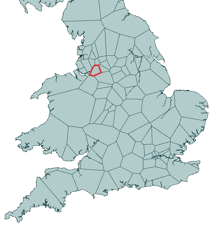
Each polygon represents an area of land closer to one particular stadium than any other. For example, the highlighted part represents that area whose closest team is Manchester United. i.e. if you live in that area, geographically your local team is Manchester United. This is just by straight line distance, by the way. It doesn’t represent a road journey.
Download
- Geographically Closest Teams (Google KML)
You’ll see that the features don’t get a label unless you click on them – so maybe you can see if you know which area is which team before clicking each area to check your guesses?
![]()
Data Integration and Statistics Generation
OK, so here’s the part where I talk about creating these statistics. Even if you came here just for the football, I think you’ll find it interesting. Plus, further down is a link to a web service for running statistics on your own data, which is quite fun.
Like I said, I used FME to do these calculations. And even though I only started out with a single list of stadiums in English football, with some Ordnance Survey open data thrown in, I was able to calculate:
- The shortest and longest distance between two stadiums (in total and per league)
- The shortest and longest cumulative distances over a season (in total and per league)
- The ratio between road and straight line distances
- The shortest route to visit every stadium (and created a GPS-compatible file to navigate that route)
- The geographic extremes of stadiums (in total) and the geographic centre of stadiums (in total and per league)
- The geographically closest team to every part of England and Wales.
I’d say that’s pretty good going – and it took me longer to write this blog than it did to actually create those numbers. That’s because FME is so great at integrating data and carrying out processing on it. If you are an FME’er and want to know how this was done, well…
Reading CSV Data
Normally this would just entail reading the data, but because the coordinates were degrees/minutes/seconds, I also had to use the DecimalDegreesCalculator transformer with a VertexCreator:
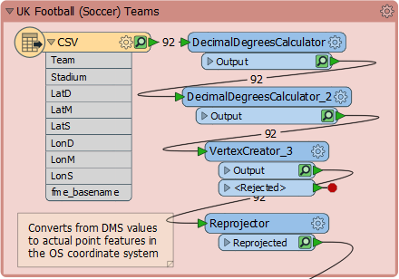
Calculating Journeys
Once I have a start/end point for each journey, the main calculation is done with the ShortestPathFinder transformer with a LengthCalculator and StatisticsCalculator:
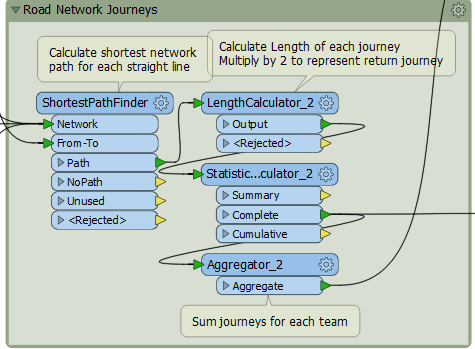
The Excel writer has a fanout set to write each league to a different sheet. The KML output has a feature type fanout for each team, with a dataset fanout per league (so one file per league, with a layer per team). But each journey gets a different value for the KML Name, so that it is like a subfolder per team, and there is a top-level document to give it a name other than doc.kml. Check out the workspace (see below). For KML users I think it’s likely to be very interesting.
Path to All Stadiums
This workspace also uses the ShortestPathFinder; but instead of being fed a series of journeys between two stadiums, it is fed a single journey between all of them:
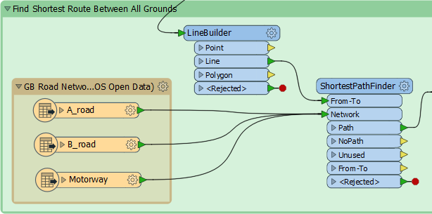
The line as built just passes through all stadiums in random order, but the ShortestPathFinder has a parameter that lets the order be changed to the optimum, so I use that.
A couple of things I found to be absolutely vital. Firstly ensure there is ample memory (close other programs if necessary) and secondly, TURN OFF FEATURE CACHING! It took way longer when I’m caching data for millions of calculations (go figure)! With the default values (10,000 iterations) it ran in a minute or so. I was intrigued to see how many iterations I could do, and if it would change the result, so I did the following:
| Iterations | Time Taken | Distance Calculated |
|---|---|---|
| 10,000 | 3 minutes, 47 seconds | 3164.0 km |
| 100,000 | 6 min, 22 sec | 3025.9 km |
| 5,000,000 (five million) | 13 min, 17 sec | 3025.9 km |
| 100,000,000 (one hundred million) | 41 min, 42 sec | 3022.7 km |
| 1,000,000,000 (one billion) | 4 hrs, 13 min, 49 sec | 3022.7 km |
After a billion iterations with no better path found, that pretty much proves the result. Still, I think this shows how increasing the processing time can produce better results, albeit with diminishing returns. I recently found a Reddit post on the shortest route between all Springfields in the US, and I would love to get hold of their dataset to try it in FME.
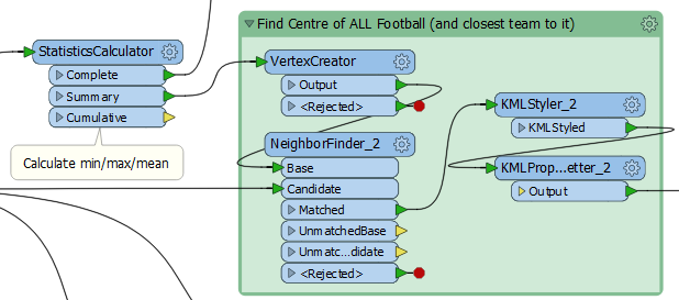
Geographic Monuments
This is perhaps the simplest workspace of all. Extract the coordinates of each feature (CoordinateExtractor) and calculate the minimum, maximum, and mean values with a StatisticsCalculator transformer. Create those points with a VertexCreator and use NeighborFinder transformer to tell me which stadium is the closest:
Geographically Closest
To generate Voronoi polygons is simple using the VoronoiDiagrammer transformer. It’s one of my favourite transformers and doesn’t get the use I think it deserves! Anyway, the main difficulty here was setting the outline of the polygons (i.e. the coastline of England and Wales). The Ordnance Survey coastline dataset returned 7,688 polygons! I had no idea there were so many islands around the coast. So I kept just the main outline and then generalized it to remove excess vertices:
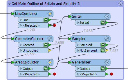
The reason for generalizing the data is that it speeds up rendering in Google Earth, and it really doesn’t affect the quality of the result.
Downloads
So if you want to try out any of these techniques, first fire up FME (if you don’t already have it running 24/7) and then try out these templates:
- Away Game Journeys
- Visiting all Stadiums (Travelling Salesman)
- Creating GPX Data
- Geographic Monuments
- Geographically Closest Teams (Voronoi Polygons)
Notice that with the Away Game Journeys workspace, you can only run one CSV file at a time, otherwise all the teams get mixed up together. Basically I need to create a group-by for the whole project, but haven’t done that yet.
![]()
Web Services
But something else that FME is also good at is serving data online as a web service, so I set that up online to let you try some of the above directly online, and even using your own data.
To try it out, step 1 is to obtain a CSV (comma-separated) dataset of British sports teams. It has to be Britain because that’s the road network I have.
Anyway, if you just want to try it out, you can download my CSV football stadium lists (the same as above) or a different dataset of Premiership rugby teams. Otherwise, create your own list using the same structure (Team,Stadium,LatD,LatM,LatS,LonD,LonM,LonS) where LatD, LatM, and LatS are the latitude in degrees, minutes and seconds, and LonD, LonM, and LonS are the longitude in degrees, minutes, and seconds.
I find that Wikipedia is great for finding coordinates:
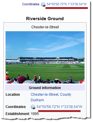
Latitude comes first, longitude is second. If the longitude coordinate is west (W) then it is a negative number. So the entry for the above would be:
Durham Cricket Club,Riverside Ground,54,50,58.72,-1,33,38.54
So make up a list of teams for any sports you like, where there are home and away fixtures. It can be national or local. Then…
Step 2: In a web browser, visit https://demos.fmeserver.com/distanceAccumulator/ – the page looks like this:
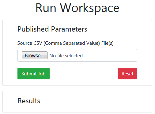
Click the Browse button to select your CSV file and click Submit Job.
Step 3: Wait a few seconds. It might not look like much is happening, but in the background FME Server is whirring away, processing your data. Very shortly you will get a link to download the results:

Click the Download Results button and there you will have it: a list of your teams in an Excel spreadsheet, in order of longest journeys, and a KML dataset for use in Google Earth that shows all of the separate fixtures and travel distances.
It’s all brought to you by the magic of FME Cloud, which processes your data using the same methods I did, but as a web service. Neat, eh?
![]()
Summary
 OK, I’m going to stop now, because this post is getting too long as it is! The football thing is fun, and I do hope some non-FME’ers find their way here for that alone. But the real point is how well FME does at data integration, data transformation, automation, web services, and much more. It really is true that it took longer to write this post than it did to generate the statistics. And thanks to my colleague Laura, the web service part only took a few minutes to put together!
I encourage FME users to check out the capabilities of transformers in the categories of Calculated Values, Integrations, and Carthographic + Reports. It’s where I got most of the functionality from for this project, and they can do a lot with just a little data.
And if anyone is like me – a spatial data wrangling, football/soccer fanatic – but hasn’t yet tried FME, well then I definitely encourage you to give it a go. It’s free to try and there are also free licenses for users such as students, non-profit organisations, and home users.
I hope you find this as interesting as I do, and feel free to let me know what you think of the data and processing techniques.


Mark Ireland
Mark, aka iMark, is the FME Evangelist (est. 2004) and has a passion for FME Training. He likes being able to help people understand and use technology in new and interesting ways. One of his other passions is football (aka. Soccer). He likes both technology and soccer so much that he wrote an article about the two together! Who would’ve thought? (Answer: iMark)